Introduction
This is a brief introduction to how to use maximum likelihood to estimate the prospect theory parameters of loss aversion (\(\lambda\)) and diminishing marginal utility (\(\rho\)) using the optim function in R. The first part is meant to go through the logic and math behind prospect theory and modeling choices. The second part goes in detail into the R code used to do the Maximum likelihood estimation plus a few of the pitfalls that you can run into. If you’re already familiar with MLE and just want the code, you can skip to the last section, which has the full code. All data and code for this page can be found here (If you’re following along, you’ll want to download “data_all_2021-01-08.csv”).
For the R portions, I’ll try to explain everything I use, but it will be helpful to be familiar with the pipe (%>%) and the baiscs of dplyr. We’ll also use purrr, and nested data/broom, but I’ll go more in depth on both of those.
This will hopefully be a series of posts going into different components of model estimation. The punchline of a lot of this will to be to use the hBayesDM package (Ahn, Haines, and Zhang 2017) which is a great hierarchical Bayesian package. Please send any errors or comments to paul.e.stillman@gmail.com.
A brief overview of prospect theory
How do people make choices involving risk and uncertainty? For instance, if someone offers you a gamble whereby they flip a coin, and if it comes up heads you win $20, but lose $18 if it comes up tails, would you accept? Do you think others would accept? One way to decide would be to simply multiply the value of the different possible outcomes by their probability, and choose the resulting option that has the highest expected value. So in our example, forgoing the gamble is equal to a value of \(\$0\), whereas electing the gamble is \(.5\cdot\$20 - .5\cdot\$18 = \$1\), which is greater than \(\$0\), so we should accept the gamble.
The problem is that most people don’t accept the gamble. Kahneman and Tversky (1979; Tversky and Kahneman 1992) developed prospect theory in order to better predict and understand how people make choices involving risk, with a particular eye to violations of expected value.1
Loss Aversion and Diminishing Marginal Utility
One insight of prospect theory is that people subjectively value gains and losses very differently than expected value would predict. Specifically, by recognizing that people display both loss aversion (where losses are weighted more heavily than equivalent gains) and diminishing marginal utility (where each subsequent dollar gained or lost is marginally less impactful than the one that came before it) – both expanded on further below – Kahneman & Tversky derived the following subjective utility function (Equation (1)):
\[\begin{equation} u(x) = \begin{cases} x^\rho & x > 0 \\ -\lambda \cdot (-x)^\rho & x \le 0 \end{cases} \tag{1} \end{equation}\]
where \(u(x)\) corresponds to the subjective utility (or subjective value) of some dollar amount \(x\).2
These functions include two parameters that correspond to the variables of interest: loss aversion (denoted by the Greek symbol lambda, \(\lambda\)) and diminishing marginal utility (denoted by the Greek symbol rho, \(\rho\))
Loss aversion
Loss aversion captures the idea that losses are more psychologically impactful than gains of equivalent size (“losses loom larger than gains”). Losing $5 feels worse than gaining $5 feels good. Loss aversion is quantified by \(\lambda\) (lambda) above: when \(\lambda = 1\), losses are weighted equivalently to gains. When \(\lambda > 1\) (as is most common), people are said to be loss averse (since they weight losses more than corresponding gains). Similarly, when \(\lambda < 1\), people underweight losses relative to gains (and often corresponds to riskier decision-making). To illustrate consider our above bet: +$20 vs. -$18. Ignoring \(\rho\) for now (by setting it to 1), and using a typical value of \(\lambda = 1.40\), we can see that \(u(20) = 20^1 = 20\) and \(u(-18) = -1.40*(18)^1 = -25.20\). Because the negative utility from the loss is of greater magnitude than the positive utility from the gain, we would expect someone for whom \(\lambda = 1.40\) to reject this gamble.
Diminishing marginal utility
Diminishing marginal utility captures the idea that gaining $10 is not quite twice as valuable as gaining $5, and losing $10 is not twice as painful as losing $5. In other words, the marginal benefit (or pain) conferred by each additional dollar earned (or lost) is not quite as beneficial (or painful) as the one that came before it. Diminishing marginal utility is quantified by \(\rho\), a quantity (generally) between 0 and 1, which introduces convexity (on the loss side) and concavity (on the gain side) to the value function (see the figure below). \(\rho = 1\) corresponds to no diminishing marginal utility, with greater diminishing marginal utility as \(\rho\) decreases.
To illustrate, consider the difference between $5 and $10: expected value would predict that $10 is valued exactly twice as much as $5, and as such people should be indifferent between a choice between $5 for certain and a 50% chance of earning either $10 or $0. But if we plug these values into our value function, we see that this is not necessarily the case. This time ignoring \(\lambda\) (by setting it to 1), and using a typical value of \(\rho = .83\), we can see that \(u(5) = 5^.83 = 3.80\) and \(u(10) = (10)^.83 = 6.76\). Here, \(u(10) < 2\cdot u(5)\) (i.e., the subjective utility of $10 is less than twice that of the subjective utility of $5).
To illustrate this, Figure 1 graphs the utility function for a given \(\lambda\) and \(\rho\):
Figure 1: Subjective Utility According to Prospect Theory (lambda = 2.6, rho = .65)
Here I’m using some fairly extreme values for lambda/rho to illustrate how the value function can deviate markedly from expected value. Were expected value accurate, people would value +5 the same magnitude as -5, and +10 would be valued twice as much as +5, indicated by the dashed line.
Both of the above parameters are reflected in this value function: loss aversion is reflected in the fact that the slope to the left of 0 is steeper than to the right of 0. Diminishing marginal utility is reflected in the fact that the utility function is concave to the right of 0, and convex to the left of 0.
Both \(\lambda\) and \(\rho\) vary greatly from person to person (and situation to situation), and indeed what we often want as researchers is to estimate these parameters for each individual person – both to understand their particular value function, as well as test if various situational/individual features shift these parameters meaningfully (e.g., Sokol-Hessner et al. 2009) – indeed, this is the entire motivation for this post. But how do we do this?
The answer is we estimate it from participants’ choices.
The Choices
To estimate these parameters, we’ll give participants a number of choices of whether to accept or reject a gamble, and then estimate their parameters from those choices. We’ll use data from one of my papers (Stillman, Krajbich, and Ferguson 2020) – you can download the data here – in which participants made 215 choices of whether to accept some gamble, or instead take some certain amount of money.
In this dataset, we have two different types of gambles, mixed and gain-only. For mixed gambles, participants had to choose whether to accept a gamble that involved the possibility of a gain (earning money) or a loss (losing money), or to reject the gamble and take $0 for certain. For instance, participants could chose to take $0 for certain, or choose to gamble, in which case they would either gain $5 or lose $3 (each outcome had probability of 50%). In gain-only gambles, participants could get some amount of money for certain (e.g., $5), or gamble and have a 50% chance of earning more (e.g., $10) and a 50% chance of earning nothing at all ($0).
In this dataset, the gamble always had two outcomes which were equally likely, 50% (this is by no means a requirement for estimating parameters from choices). There were 165 mixed gambles (which participants completed first) and 50 gain-only gambles. Across 3 studies, we have 652 participants. Here’s what the data look like:
The data are in long format, meaning 1 row per choice, with columns for study (1 to 3), subject (N = 652), and trial (215 trials, starts at 9 due to instructions screens and practice). Gamble type indicates whether it was a mixed gamble (“gain_loss”) or a gain-only gamble (“gain_only”). “gain,” “loss,” and “cert” (short for “certain”) correspond to the amount of money that would be gained or lost if the participants chose to gamble and won, gambled and lost, or if the participants took the certain amount (respectively – note that cert is always 0 for the mixed gambles and loss is always 0 for the gain-only gambles). took_gamble is 1 if participants chose to gamble, 0 otherwise (participants were not given feedback about the gamble outcome).
From Choices to Likelihoods
Okay, so now we have a whole bunch of choices for each participant. The broad strokes version of what we’re going to do is:
A. select a candidate value of \(\rho\) and \(\lambda\) for a given participant (we’ll start with values from past research) B. see how well those values capture the participants’ 215 choices C. choose new values of \(\rho\) and \(\lambda\) and see if those new values do better or worse
and then repeat that a whole bunch of times until we have values we think best capture the choices. Step C is mostly going to be handled under-the-hood by the maximum likelihood algorithm, and step A is generally taken from prior research (here we will use the average values reported in Sokol-Hessner et al. 2009) so for now let’s focus on step B: evaluating how well a given \(\rho\) and \(\lambda\) correspond to participants’ choices.
The first thing that we need is a way to translate a candidate \(\rho\) and \(\lambda\) into a probability of accepting or rejecting the gamble. For this, we’ll use a function that takes as input the difference in subjective utility between the two options: \(u(accept) - u(reject)\):
\[\begin{align} u(reject) &= u(certain) \\ u(accept) &= .5 \cdot u(gain) + .5\cdot u(loss) \\ u(\text{gamble_cert_diff}) = u(accept) - u(reject) &= (.5\cdot u(gain) + .5 \cdot u(loss)) - u(certain) \tag{2} \end{align}\]
(here, u(reject) = u(certain) because if you reject the gamble you instead get the certain amount). We’ll next use this gamble_cert_diff (i.e., the difference in subjective utility of the two choices) to determine how likely one is to accept or reject. Specifically, we’ll use the function in Equation (3)
\[\begin{equation} p(accept) = \frac{1}{1 + exp(-\mu \cdot \text{gamble_cert_diff})} \tag{3} \end{equation}\]
(Ignore the \(\mu\) for a minute, we’ll get back to that in a second). In case that equation looks intimidating to you, I think it’s much intuitive what is going on when you graph it (Figure 2):
Figure 2: Probability of accepting the gamble as a function of the difference in subjective utility of accepting vs. rejecting the gamble.
Graphically, this should (hopefully) make more sense: when the subjective utilities of the both options (accept or reject the gamble) are the same (the difference is 0), people are equally likely to take either option (50%). As the subjective utility of accepting the gamble increases relative to passing it (i.e., as we move rightward from 0), the likelihood of accepting the gamble increases, until it asymptotes at 1 (similarly, as passing the gamble gets more attractive relative to accepting, moving left-ward from 0, the probability of gambling gets lower and lower until it asymptotes at 0). In this way, we’ve translated our \(\lambda\) and \(\rho\) values (which are used to compute the subjective utilities) to a probability of choosing the gamble, which in turn will allow us to evaluate how well our proposed \(\lambda\) and \(\rho\) values actually capture a given set of choices.
But what’s \(\mu\) (mu)? As it turns out, this is a third parameter that we will estimate for each person. It reflects how sensitive people are to differences in subjective utility. \(\mu = 0\) means choices are random, and as mu increases the function becomes more sharp at 0 (Figure 3):
Figure 3: Probability of accepting the gamble for different values of mu.
Someone using a rule such as “accept gambles with positive expected value” will have a high value for \(\mu\), whereas those people who are less consistent in their choices will have a lower value for \(\mu\). (While it is very useful include \(\mu\) to estimate the other parameters, it often receives less attention by researchers, who usually are more interested in \(\lambda\))
Okay! So! For some proposed value of \(\lambda\), \(\rho\), and \(\mu\), we have a way to change each decision into a probability-to-accept (i.e., by using \(\lambda\) and \(\rho\) to calculate the subjective utility of accepting and of passing, and plugging the difference into the above formula along with \(\mu\)). The next step is to simply compare the actual choice to what the model predicts given the parameters. We use the following likelihood function to do so:
\[\begin{equation} \text{trial likelihood} = [p(accept)]^y \cdot [1-p(accept)]^{1-y} \tag{4} \end{equation}\]
where y = 1 if the participant chose the gamble, and y = 0 if they did not. To illustrate, suppose \(p(accept) = .75\), and the participant indeed accepted the gamble (so \(y = 1\)). In this case, the likelihood for this trial is:
\[\begin{align} [p(accept)]^y \cdot [1-p(accept)]^{1-y} &= \\ .75^1 \cdot (1-.75)^{1-1} &= \\ .75^1 \cdot (.25)^0 &= .75 \end{align}\]
On the other hand, if participants rejected the gamble (\(y = 0\)), then the likelihood is \(.75^0 * (1-.75)^{1-0} = .25\).
Overall, higher likelihood corresponds to a better fit of your parameters. If a certain set of parameters assigns a \(p(accept)\) of .8, and the participant indeed chose to gamble, they will have a higher likelihood than a set of parameters for which \(p(accept) = .75\) (.8 vs .75). But if the participant chose to pass, then the likelihood will be higher for the model with \(p(accept) = .75\) (.25 vs. .2). In other words, if the model is ‘right,’ it gets more credit (i.e., likelihood) for being confident, but if it is wrong it gets penalized for being over-confident.
Note that the above calculations are just the probability/likelihood for a single trial given some set of parameters. What we want is the probability across all 215 of a subjects’ trials – in other words, the joint probability. To get this (the “full” likelihood), we assume each trial is independent, and then multiply the likelihood of each of the 215 trials together (recall from intro probability that if two events are independent, their joint probability is just the probability of each event multiplied together). So we take each of the above trial probabilities and multiply them all together (if the following equation is confusing you can just skip it we’re about to deal with something a bit more manageable):
\[\begin{equation} Likelihood = \prod_{i = 1}^{215} [p(accept)_i]^{y_i} \cdot [1-p(accept)_i]^{1-y_i} \tag{5} \end{equation}\] where \(i\) represents the trial (from 1 to 215), \(y_i\) represents the choice made on trial \(i\), and \(p(accept)_i\) represents the predicted probability of acceptance on trial \(i\). For a few reasons, however, we’re going to use a slight variant of that which changes two things. First, we’re going to multiply it by negative 1 (most optimizers actually minimize a value, so rather than trying to maximize likelihood we will minimize negative likelihood). Second, we’re going to take the log of it instead to get log likelihood:
\[\begin{equation} LL = -\sum_{i = 1}^{215} y_i \cdot log[p(accept)_i] + (1-y_i) \cdot (1-log[p(accept)_i]) \tag{6} \end{equation}\] (recall that for logarithms, exponentials become multiplication, and multiplication becomes addition, if you need a refresher on logarithms, I suggest the log section on this excellent page). This number represents the negative log likelihood across all trials for a given set of parameters \(\lambda\), \(\rho\), and \(\mu\). Remember above we said we were going to try a whole bunch of different combinations and choose the one that’s best. Maximum Likelihood refers to an algorithm that repeats the above processes many times, changing the parameters each time, in order to find the parameters that maximize the likelihood (or, rather, minimize negative likelihood). The output is the parameters that best capture a participants’ choices (the ones with the highest likelihood across all choices).
To recap, let’s quickly summarize what that whole process looks like. The following is what maximum likelihood is for fitting a given individuals’ choices:
- Choose some initial starting values for parameters \(\lambda\), \(\rho\), and \(\mu\) (we’ll take these from past research)
- Use those parameters to calculate, for each trial, the subjective utility of the gain, loss and certain option using the equation \(u(x) = \begin{cases} x^\rho & x > 0 \\ -\lambda \cdot (-x)^\rho & x \le 0 \end{cases}\)
- Use values from (2) to calculate the difference in subjective utility for each trial \(u(\text{gamble_cert_diff}) = u(accept) - u(reject) = (.5\cdot u(gain) + .5\cdot u(loss)) - u(certain)\)
- For each gamble, enter this subjective utility difference and \(\mu\) into the following equation to get the probability of accepting the gamble: \(p(accept) = \frac{1}{1 + exp(-\mu \cdot \text{gamble_cert_diff})}\)
- Calculate the negative log likelihood across all trials: \(LL = -\sum_{i = 1}^{215} y_i \cdot p(accept)_i + (y_i-1) \cdot (1-p(accept)_i)\)
- If the LL in this iteration does not differ substantially from the previous iteration, finish. Otherwise, propose new parameter values and return to step 2. As noted above, the specific stopping rules and parameter proposals are mostly handled by the algorithms implementing maximum likelihood (if you are interested in going deeper into the details of these algorithms, check out Myung 2003).
And that’s all there is to it! Now let’s implement it in R.
Maximum Likelihood in R
To implement this in R, we use the optim function, which is R’s built-in optimizer.3 To keep things a bit more manageable, we’ll start with just one participant.
library(tidyverse)
data_clean <- read_csv('data_all_2021-01-08.csv')

# select on a single subject:
data_s1_101 <- data_clean %>% filter(study == 'study_1', subject == 101)
paged_table(data_s1_101)
The first thing that we’ll do is write functions that correspond to the equations in steps 2-4 above:
# Step 2: Calculate subjective utility given lambda/rho (Equation (1) above)
# takes a vector of values and parameters and returns subjective utilities
calc_subjective_utility <- function(vals, lambda, rho) {
  # if the value is greater than or equal to 0, return the value raised to rho.
  # Otherwise return -lambda times the value raised to rho
  # (we multiply the value by -1 so that we always get a positive
  # number when we raise it to rho)
  ifelse(vals >= 0, vals^rho, -lambda * ((-vals)^rho))
}

# Step 3: Calculate utility difference from vectors of gains,
# losses, and certainty (Equation (2) above)
calc_utility_diff <- function(su_gain, su_loss, su_cert) {
  # gamble subjective utility (su) = .5 times gain subjective utility plus
  # .5 times loss subjective utility. Then take the difference with certain
  (.5*su_gain + .5*su_loss) - su_cert
}

# Step 4: Calculate the probability of accepting a gamble,
# given a difference in subjective utility and mu (Equation (3) above)
calc_prob_accept <- function(gamble_cert_diff, mu) {
  (1 + exp(-mu * (gamble_cert_diff)))^-1
}
Let’s walk through one iteration of the above steps (1-6) manually before applying the maximum likelihood algorithm. For the starting value, we’ll use \(\lambda = 1.40\), \(\rho = .83\), and \(\mu = 2.57\) (the average from Study 1 from Sokol-Hessner et al. 2009). The first 5 steps look like this:
# Step 1: choose starting parameters (here we take some from previous research)
lambda_par <- 1.4
rho_par <- .83
mu_par <- 2.57
data_s1_101_su <- data_s1_101 %>%
  # (mutate = add variables)
  mutate(
    # Step 2: calculate subjective utility:
    cert_su = calc_subjective_utility(cert, lambda_par, rho_par),
    loss_su = calc_subjective_utility(loss, lambda_par, rho_par),
    gain_su = calc_subjective_utility(gain, lambda_par, rho_par),
    # Step 3: calculate the difference in
    # subjective utility between choices:
    gamble_cert_diff = calc_utility_diff(gain_su, loss_su, cert_su),
    # Step 4: calculate the probability of accepting
    prob_accept = calc_prob_accept(gamble_cert_diff, mu = mu_par),
    # Step 5a: calculate log likelihood on each trial
    log_likelihood_trial = took_gamble*log(prob_accept) +
      (1-took_gamble)*log(1-prob_accept))

# Step 5b: calculate overall Negative log-likelihood as the sum of all trial likelihoods times minus 1:
-sum(data_s1_101_su$log_likelihood_trial)
[1] 76.68009So in this case, the negative log likelihood is 76.6800899. We’ll then repeat this process trying out different parameter values, and take whichever has the lowest negative log likelihood (i.e., the highest likelihood).
Using optim in R
The optim function requires, at minimum, starting parameter values (par) and a function to optimize (fn). What optim will do is call the function fn many times, varying the parameter values par in an attempt to minimize the ouptut of the fn function (which, recall, is negative log likelihood).
The bulk of coding goes into writing fn correctly. fn must be a function with the following properties:
- At least one argument in the function call must be
par– which will be a list of the different parameters to be optimized. This takes the formpar = c(par_1, par_2, par_3)(see below) - The function must return a single value – in this case the negative log likelihood – which
optimwill attempt to minimize by altering the parameter values.
To do this, we just need to modify the above code slightly so that it conforms with these requirements. Once we have written the above function, we can call it with optim via the call optim(par = c(1.4,.83,2.57), fn = function_to_minimize, ...) where par allows us to set starting values of the parameters, fn is the function to minimize, and the ... will allow us to send other variables the function requires – for our purposes, this will just be the dataframe that has all of the subjects choices.
This will all hopefully be more clear with an example, again looking at our single participant:
# the function to minimize:
minimize_LL_prospect_v1 <- function(df, par) {
  # takes as input par, which is expected to be of the form c(lambda, rho, mu)
  # takes also a dataframe of gambles and choices (in this example, our single subject)
  lambda_par <- par[1]
  rho_par <- par[2]
  mu_par <- par[3]
  df_updated <- df %>%
    # (mutate = add variables)
    mutate(
      # Step 2: calculate subjective utility:
      cert_su = calc_subjective_utility(cert, lambda_par, rho_par),
      loss_su = calc_subjective_utility(loss, lambda_par, rho_par),
      gain_su = calc_subjective_utility(gain, lambda_par, rho_par),
      # Step 3: calculate the difference in
      # subjective utility between choices:
      gamble_cert_diff = calc_utility_diff(gain_su, loss_su, cert_su),
      # Step 4: calculate the probability of accepting
      prob_accept = calc_prob_accept(gamble_cert_diff, mu = mu_par),
      # Step 5: calculate log likelihood
      log_likelihood_trial = took_gamble*log(prob_accept) +
        (1-took_gamble)*log(1-prob_accept))

  # Now we simply return the negative log-likelihood:
  -sum(df_updated$log_likelihood_trial)
}

# the optim call, with starting values:
optim(par = c(1.24, .83, 2.57),
      fn = minimize_LL_prospect_v1,
      df = data_s1_101)
$par
[1] 1.4383057 0.9481158 1.2928924

$value
[1] 70.49725

$counts
function gradient
      94       NA

$convergence
[1] 0

$message
NULL
If you haven’t done anything like this before, then congrats – you’ve just fit your first computational model. Exhilarating. optim outputs a list (here and below, the grey box corresponds to the output of the code). The two fields you’ll want to look at are $par and $convergence. $par gives the optimized parameters: in this case \(\lambda = 1.44\), \(\rho = .95\), and \(\mu = 1.29\), which seem reasonable enough (we’ll go through checking model fit later). $convergece lets you know if everything went alright: if this is 0 (as it is here) it means that the algorithm completed successfully.
As I said above: exhilarating. You’re probably so excited you can’t wait to do another, and far be it from me to hold you back, so let’s do it again with another subject. Specifically, we’ll do subject 105 from study 1:
data_s1_105 <- data_clean %>% filter(study == 'study_1', subject == 105)
# do the same optim call again, just changing the df input:
optim(par = c(1.24, .83, 2.57),
      fn = minimize_LL_prospect_v1,
      df = data_s1_105)
$par
[1] -718.22647302    0.11504388    0.01135451

$value
[1] 40.67213

$counts
function gradient
     502       NA

$convergence
[1] 1

$message
NULL
Hrmm. That doesn’t look so good. Recall above we said that \(\lambda = 1\) means that losses are equivalent to gains, \(\lambda > 1\) corresponds to loss aversion, and \(\lambda < 1\) means that people weight gains more heavily than losses (e.g., someone might accept a +$5/-$6 gamble, for instance). A \(\lambda = -718.22\) would mean that someone values a loss of $1 the same as a gain of $718.22.
In other words, unlike with subject 101, these parameters make no sense at all (I’m focusing on \(\lambda\) here but \(\rho\) and \(\mu\) aren’t much better). You’ll also note that the $convergence is equal to 1, which means the algorithm stopped because it had done x number of iterations, rather than because it found the minimum value.4
What we want to do here is to tell optim to not allow \(\lambda\) or our other parameters to be less than 0, because in our model negative values of these parameters don’t make sense. To do this, we need to change two options in our function call: first, we need to add lower = c(0,0,0) which tells the algorithm that the lower bounds for our 3 parameters are 0 (we’ll also add upper = c(Inf,Inf,Inf) so that we’re precise about our bounds). Next, because the default optimizer that optim uses can’t actually handle bounds, we need to change the optimizer by adding method = 'L-BFGS-B', which is an algorithm that can handle bounds (more info available on these different algorithms by checking ?optim).
So let’s try that:
optim(par = c(1.24, .83, 2.57),
      fn = minimize_LL_prospect_v1,
      df = data_s1_105,
      method = 'L-BFGS-B',
      lower = c(0,0,0),
      upper = c(Inf, Inf, Inf))
$par
[1] 0.0000000 0.8156675 1.6250083

$value
[1] 48.92777

$counts
function gradient
      13       13

$convergence
[1] 0

$message
[1] "CONVERGENCE: REL_REDUCTION_OF_F <= FACTR*EPSMCH"
Well… that looks a little better? At least \(\rho\) and \(\mu\) look a bit more normal, though obviously a \(\lambda\) of 0 still isn’t ideal – it basically means that this person views all loses as equivalent to $0 (in other words, this participant is totally insensitive to losses). To investigate this, we can look at their data (something we probably should have done first) – specifically, what did their choices look like for the mixed gambles (i.e., the gambles for which loss was a possibility) and the gain-only gambles?
data_s1_105 %>%
  group_by(gamble_type) %>%
  summarise(num_gambles_accepted = sum(took_gamble), num_choices = n())
# A tibble: 2 x 3
  gamble_type num_gambles_accepted num_choices
  <chr>                      <dbl>       <int>
1 gain_loss                    164         165
2 gain_only                     28          50
Ah, well now this makes a bit more sense: of the 165 choices between receiving $0 and a gamble that involved a possibility of a loss, this participant gambled 164 times. In this light, a \(\lambda\) of 0 makes a bit more sense – regardless of the loss the participant chose to gamble 99.4% of the time (whereas in the gain-only trials they seem to have behaved more normally). In that light, it does appear that their choices are unresponsive to the magnitude of the loss, and a \(\lambda\) of 0 might make a bit more sense. It is of course unlikely that someone would actually be totally insensitive to losses. There are a few possibilities of what happened here. First, it’s possible that we just didn’t give them losses large enough to see them rejecting gambles. So perhaps if this person were given gambles that had more extreme losses we would get a more sensible value for \(\lambda\) (e.g., +$5/-$50). This is actually a more general problem: for your model to make sense, you need to make sure the choices you select are likely to get enough variance to actually meaningfully estimate the parameters (i.e., you want gambles where people will make a range of choices).
The second possibility, of course, is that sometimes participants just really don’t want to do your task, and may just be clicking through it (or, more charitably, that they were confused about the instructions). My money is on this one here – the one gamble they passed was +$14/-$5.25, a gamble which was accepted by 88% of participants.
Okay, whatever, sometimes that happens, let’s just move on. Before we loop it for every participant, let’s do a sanity check and try this new method (with bounds) with our first participant (it should give us similar values as above):
optim(par = c(1.24, .83, 2.57),
      fn = minimize_LL_prospect_v1,
      df = data_s1_101,
      method = 'L-BFGS-B',
      lower = c(0,0,0),
      upper = c(Inf, Inf, Inf))
Error in optim(par = c(1.24, 0.83, 2.57), fn = minimize_LL_prospect_v1, : L-BFGS-B needs finite values of 'fn'
Shit. What happened? I’ll spare you all of the debugging code and tell you that the algorithm fails with parameters = c(2.022408, 1.450688, 2.519166).5 Let’s plug those parameter numbers in and see if that tells us anything:
lambda_par <- 2.022408
rho_par <- 1.450688
mu_par <- 2.519166
data_s1_101_su <- data_s1_101 %>%
  # (mutate = add variables)
  mutate(
    # Step 2: calculate subjective utility:
    cert_su = calc_subjective_utility(cert, lambda_par, rho_par),
    loss_su = calc_subjective_utility(loss, lambda_par, rho_par),
    gain_su = calc_subjective_utility(gain, lambda_par, rho_par),
    # Step 3: calculate the difference in
    # subjective utility between choices:
    gamble_cert_diff = calc_utility_diff(gain_su, loss_su, cert_su),
    # Step 4: calculate the probability of accepting
    prob_accept = calc_prob_accept(gamble_cert_diff, mu = mu_par),
    # Step 5: calculate log likelihood
    log_likelihood_trial = took_gamble*log(prob_accept) +
      (1-took_gamble)*log(1-prob_accept))

tail(data_s1_101_su, n = 10) %>% paged_table()
Scroll to the right in the table above (click the arrow in the top-right corner). Our problem stems from the NaN in the log likelihoods. To investigate further, lets focus on those:
# keep only rows for which the log likelihood is NaN or -Inf
data_nan <- data_s1_101_su %>%
  filter(!is.finite(log_likelihood_trial))

paged_table(data_nan)
From that, we can see that there are 20 gambles that have ‘NaN’ or -Inf as the log likelihood. What all of these have in common is that the probability of accepting a gamble (using these parameter values) is 1.
The reason that these parameter values are 1 is due to rounding in R. Our probability to accept function (Figure 2 above) asymptotes at 1 and 0, but only actually reaches those values at +/- infinity. The problem is that the difference in subjective utility (given the parameters) is large enough that it leads to a probability of accepting that is close enough to 1 as to be rounded up to 1. This in turn causes took_gamble*log(prob_accept) + (1-took_gamble)*log(1-prob_accept) to be undefined because log(0) = negative infinity.
There’s a few ways to handle this, but the one we’ll use is to change the function we are optimizing so that it subtracts or adds a very small number when the probability of accepting has been rounded to 1 or 0 (respectively):
minimize_LL_prospect <- function(df, par) {
  lambda_par <- par[1]
  rho_par <- par[2]
  mu_par <- par[3]
  df_updated <- df %>%
    mutate(
      cert_su = calc_subjective_utility(cert, lambda_par, rho_par),
      loss_su = calc_subjective_utility(loss, lambda_par, rho_par),
      gain_su = calc_subjective_utility(gain, lambda_par, rho_par),
      gamble_cert_diff = calc_utility_diff(gain_su, loss_su, cert_su),
      prob_accept = calc_prob_accept(gamble_cert_diff, mu = mu_par),
      # Recode the probability of acceptance, such that if it's 1, subtract
      # a very small amount, and if it's 0 add a very small amount"
      prob_accept_rc = case_when(prob_accept == 1 ~ 1-.Machine$double.eps,
                                 prob_accept == 0 ~ 0+.Machine$double.eps,
                                 TRUE ~ prob_accept),
      # calculate log likelihood on this slightly altered amount
      log_likelihood_trial = took_gamble*log(prob_accept_rc) +
        (1-took_gamble)*log(1-prob_accept_rc))

  -sum(df_updated$log_likelihood_trial)
}

# with this updated function, we can try again:
optim(par = c(1.24, .83, 2.57),
      fn = minimize_LL_prospect,
      df = data_s1_101,
      method = 'L-BFGS-B',
      lower = c(0,0,0),
      upper = c(Inf, Inf, Inf))
$par
[1] 1.4382777 0.9480954 1.2928266

$value
[1] 70.49725

$counts
function gradient
      21       21

$convergence
[1] 0

$message
[1] "CONVERGENCE: REL_REDUCTION_OF_F <= FACTR*EPSMCH"
Hooray it works! And if you compare it with the other optimizer we used above, the answers are almost identical, which is a nice sanity check.
Before we move on to looping through everyone, there is another error that can come up relating to the estimation of \(\rho\). Occasionally the algorithm will try a parameter value for \(\rho\) that is too large, and then when we go to calculate the subjective utility \(x^\rho\) that value will be large enough that R treats it as infinity, which causes all of the subsequent calculations to be undefined. There are a few ways to address this problem, but for now what we’re going to do is put a cap on the size of \(\rho\). \(\rho\) is intended in our model to be an exponential downweight, which means that values larger than 1 don’t make a ton of sense. However, it is conceivable that someone might have \(\rho\) of larger than 1 (e.g., viewing $1 as trivial and only caring when it gets to larger values), so we don’t want a hard ceiling at 1. Instead we’ll set an upper limit of \(\rho = 10\). It’s an arbitrary decision, but should keep us from getting infinities that break our code:
data_s3_1038 <- filter(data_clean, study == 'study_3', subject == 1038)
# the optim call, with starting values:
optim(par = c(1.24, .83, 2.57),
      fn = minimize_LL_prospect,
      df = data_s3_1038,
      method = 'L-BFGS-B',
      lower = c(0,0,0),
      upper = c(Inf, 10, Inf))
$par
[1] 0.8926703527 0.0007285268 1.1297095853

$value
[1] 146.9664

$counts
function gradient
      68       68

$convergence
[1] 52

$message
[1] "ERROR: ABNORMAL_TERMINATION_IN_LNSRCH"
Notice that this still doesn’t converge (and that’s going to be the case for some people, especially when using maximum likelihood), but at least it won’t cause our code to error out when we loop it (also later when we introduce multiple starting points and impose more bounds this participant does actually converge).
Now that we’ve fixed up those bugs, we can loop this over every participant.
Looping over multiple participants
So now we want to loop over every participant and use optim to fit their parameters. There are two ways to do this: a for loop (easy, inelegant, lame) or by using nest and map (slightly more complicated, elegant, extremely cool). We’re gonna do the latter, because it can really help when doing modeling, but if you want I’ve included some inelegant code at the bottom to do the same thing with a for loop.
Nesting in R
The first thing we’re going to do here is nest our data such that each line is a subject that has only three columns: study, subject, and data, with this last column being a list-column that contains the full dataset for each participant. I’ll try to give a succinct explanation of nested data, but if you want to go more in depth see here or here.
data_nested <- data_clean %>%
  nest(data = -c(study, subject)) # nest everything within study/subject

data_nested
# A tibble: 652 x 3
   study   subject data
   <chr>     <dbl> <list>
 1 study_1     101 <tibble [215 x 6]>
 2 study_1     102 <tibble [215 x 6]>
 3 study_1     103 <tibble [215 x 6]>
 4 study_1     104 <tibble [215 x 6]>
 5 study_1     105 <tibble [215 x 6]>
 6 study_1     106 <tibble [215 x 6]>
 7 study_1     107 <tibble [215 x 6]>
 8 study_1     108 <tibble [215 x 6]>
 9 study_1     109 <tibble [215 x 6]>
10 study_1     110 <tibble [215 x 6]>
# ... with 642 more rows
# optim_all <- data_nested %>%
# mutate(optim_output = map(data, ~ optim(par = c(1.24, .83, 2.57), fn = minimize_LL_prospect_v1, df = .)))
So now we’ve gone from a dataframe where each row is a gamble to one where each row is a subject, with a variable data that contains everything else for that subject. So if we look at the first data:
data_nested$data[[1]] %>% paged_table()
This is just what we had above – a single dataframe for the participant corresponding to all of their choices. The reason for doing this is it allows us to elegantly run the same code (i.e., the same optim call) to many different datasets at once by applying the same function to every row (i.e., every participant).
The way we run the same optim call for each row is using the map family of functions from the purrr package (one of the tidyverse packages). These functions take a list as input, run some user-specified function on each element in the list, and return a value. map returns a list, map_dbl returns a double, map_chr returns a character string, etc.
To illustrate, consider a simple example where we just want to know how many gambles each participant accepted, we can use the following code to find that out:
data_nested %>%
  mutate(num_gambles_accepted = map_dbl(data, ~ sum(.$took_gamble)))
# A tibble: 652 x 4
   study   subject data               num_gambles_accepted
   <chr>     <dbl> <list>                            <dbl>
 1 study_1     101 <tibble [215 x 6]>                   86
 2 study_1     102 <tibble [215 x 6]>                   15
 3 study_1     103 <tibble [215 x 6]>                   77
 4 study_1     104 <tibble [215 x 6]>                   98
 5 study_1     105 <tibble [215 x 6]>                  192
 6 study_1     106 <tibble [215 x 6]>                  101
 7 study_1     107 <tibble [215 x 6]>                  118
 8 study_1     108 <tibble [215 x 6]>                   38
 9 study_1     109 <tibble [215 x 6]>                   82
10 study_1     110 <tibble [215 x 6]>                  141
# ... with 642 more rows
Let me unpack that function call a bit. First, we’re using mutate because we want to make a new variable num_gambles_accepted. We use map_dbl because we know we’re getting a numerical value as output. data here is the field that contains all the choices for each participant (an entire dataframe is stored, for each row, in this field). The map family of functions work by taking a list and applying the function to every element of the list (it’s similar to the apply family of functions in base R), so we provide map_dbl with the column data, and have it apply some function to each dataframe (one per subject). So map_dbl(data, ...) means apply a function to each element of data (i.e., each participants’ dataframe of choices). Next we have to tell it what function to apply. The ~ means we’re going to be making a custom function here. The .$took_gamble is a little ugly, but here . just refers to the field being passed to the function. Since we’re passing a dataframe, this is basically the same as saying df$took_gamble. Then the sum is just the sum function.
So to summarize, this call basically says "for every row in this dataframe, take the data field (which itself contains all choices that each participant made), then sum all values in the took_gamble field, and save it as a new variable num_gambles_accepted.
optim using nest
Hopefully that wasn’t too terribly confusing. Next we’re just gonna do the same thing but using optim instead of summing the number of gambles accepted. This time we’ll use map rather than map_dbl, since optim returns a list. This list will be added as a new variable optim_out (note that, depending on your computer, this might take a while to run):
data_optim <- data_nested %>%
  mutate(optim_out = map(data, ~ optim(par = c(1.24, .83, 2.57),
                                               fn = minimize_LL_prospect,
                                               df = .,
                                               method = 'L-BFGS-B',
                                               lower = c(0,0,0),
                                               upper = c(Inf, 10, Inf))))

data_optim
# A tibble: 652 x 4
   study   subject data               optim_out
   <chr>     <dbl> <list>             <list>
 1 study_1     101 <tibble [215 x 6]> <named list [5]>
 2 study_1     102 <tibble [215 x 6]> <named list [5]>
 3 study_1     103 <tibble [215 x 6]> <named list [5]>
 4 study_1     104 <tibble [215 x 6]> <named list [5]>
 5 study_1     105 <tibble [215 x 6]> <named list [5]>
 6 study_1     106 <tibble [215 x 6]> <named list [5]>
 7 study_1     107 <tibble [215 x 6]> <named list [5]>
 8 study_1     108 <tibble [215 x 6]> <named list [5]>
 9 study_1     109 <tibble [215 x 6]> <named list [5]>
10 study_1     110 <tibble [215 x 6]> <named list [5]>
# ... with 642 more rows
From here we can extract the relevant data from the output: whether or not the algorithm converged and the 3 parameters:
data_optim_pars <- data_optim %>%
  mutate(convergence = map_dbl(optim_out, 'convergence'),
         pars = map(optim_out, 'par'),
         lambda = map_dbl(pars, ~ .[1]),
         rho = map_dbl(pars, ~ .[2]),
         mu = map_dbl(pars, ~ .[3]))

paged_table(data_optim_pars)
(To see convergence and model parameters for each participant, click the arrow in the upper-right-hand corner of the table). If we check for convergence (e.g., sum(data_optim_pars$convergence !=0)), we find that only 8 people failed to converge, which isn’t bad in a sample of 652! The next thing to do is look at the distribution of our parameters to see if they make sense (Figure 4):
library(patchwork)
hist_lambda <- data_optim_pars %>%
  filter(convergence == 0) %>%
  ggplot(aes(x = lambda)) +
  geom_histogram() +
  labs(title = 'lambda')
hist_rho <- data_optim_pars %>%
  filter(convergence == 0) %>%
  ggplot(aes(x = rho)) +
  geom_histogram() +
  labs(title = 'rho')
hist_mu <- data_optim_pars %>%
  filter(convergence == 0) %>%
  ggplot(aes(x = mu)) +
  geom_histogram() +
  labs(title = 'mu')

hist_lambda + hist_rho + hist_mu
Figure 4: Histograms of lambda, rho, and mu.
That looks… well \(\rho\) looks kind of okay, the other two have some pretty crazy outliers. In the next section we’ll impose some more constraints on our parameters to make them a bit more sensible. Specifically, we’ll use lower = c(.01, .01, .01) and upper = c(20, 10, 20) as the constraints. Where did I get these numbers? I asked a friend whose lab does these things and he said those are what his lab uses. In the future, we’ll instead use hierarchical Bayesian analyses which will allow us to set up sensible priors for our parameters, which is a more elegant way around the problem of “hrmm I have some huge outliers and they probably aren’t right.”
Multiple starting points
One last wrinkle that is important to note: the starting point we provide can impact the results. The technical way to describe this is that the algorithm sometimes finds local minima, rather than global minima, and the local minima it finds is based on where we start it. Below, we’ll use four different starting points rather than just one.6
Because this can take a while, I’m going to use the furrr package, which allows for parallel computing in conjunction with purrr (i.e., the package that contains the map functions). If you don’t want to mess around with this, you can delete the first two lines of code here, and replace future_map with just map (it will take 4 times as long as the above code, however). You can also download the output, “data_optim_quad.rds,” here.
library(furrr)
# set workers to the number of cores in your machine (4 here)
future::plan(multisession, workers = 4)
# if not using multicore, you can ignore the above
# lines and replace the `future_map` with `map`
data_optim_quad <- data_nested %>%
  mutate(optim_out_1 = future_map(data, ~ optim(par = c(1.24, .83, 2.57),
                                               fn = minimize_LL_prospect,
                                               df = .,
                                               method = 'L-BFGS-B',
                                               lower = c(.01,.01,.01),
                                               upper = c(20, 10, 20))),
         optim_out_2 = future_map(data, ~ optim(par = c(1, 1, 1),
                                               fn = minimize_LL_prospect,
                                               df = .,
                                               method = 'L-BFGS-B',
                                               lower = c(.01,.01,.01),
                                               upper = c(20, 10, 20))),
         optim_out_3 = future_map(data, ~ optim(par = c(2, 1, .9),
                                               fn = minimize_LL_prospect,
                                               df = .,
                                               method = 'L-BFGS-B',
                                               lower = c(.01,.01,.01),
                                               upper = c(20, 10, 20))),
         optim_out_4 = future_map(data, ~ optim(par = c(1.5, .83, 4.22),
                                               fn = minimize_LL_prospect,
                                               df = .,
                                               method = 'L-BFGS-B',
                                               lower = c(.01,.01,.01),
                                               upper = c(20, 10, 20))))
Now instead of 1 output we have 4 outputs. What we need next is a function that compares them and takes the one with the best fit. To do that we’ll select all models that converged, and take the one with the lowest log likelihood. Then we’ll extract the convergence and parameters from that:
# takes a list of models, returns the one with the lowest LL that also converged
evaluate_model <- function(model_list) {
  # This code is fairly ugly. Sorry.
  names(model_list) <- str_c('m', 1:length(model_list))
  models_tibble <- as_tibble(model_list)

  convergence_mat <- models_tibble %>%
    summarise(across(everything(), ~ map_dbl(., 'convergence'))) # convergence
  ll_mat <- models_tibble %>%
    summarise(across(everything(), ~ map_dbl(., 'value'))) # log likelihood

  ll_mat[convergence_mat != 0] <- NA # set LL of non-converging models to be NA
  lowest_likelihood <- apply(ll_mat, 1, which.min) # choose the minimum LL from each row

  index_mat <- matrix(c(1:nrow(models_tibble), lowest_likelihood), ncol = 2, byrow=FALSE)
  as.matrix(models_tibble)[index_mat] # for each row, return the optim output that had minimum LL
}

data_optim_quad_pars <- data_optim_quad %>%
  mutate(best_model = evaluate_model(list(optim_out_1, optim_out_2, optim_out_3, optim_out_4)),
         convergence = map_dbl(best_model, 'convergence'),
         pars = map(best_model, 'par'),
         lambda = map_dbl(pars, ~ .[1]),
         rho = map_dbl(pars, ~ .[2]),
         mu = map_dbl(pars, ~ .[3]))
If you poke around the above output, you’ll see that having multiple starting points gets us two things. First, now every participant is successfully converging in at least one of their models (instead of having to drop the 8 people who didn’t converge), and in a few places we have better fitting parameters. If we look at our histograms again, here’s what we see (5):
library(patchwork)
hist_lambda <- data_optim_quad_pars %>%
  filter(convergence == 0) %>%
  ggplot(aes(x = lambda)) +
  geom_histogram() +
  labs(title = 'lambda')
hist_rho <- data_optim_quad_pars %>%
  filter(convergence == 0) %>%
  ggplot(aes(x = rho)) +
  geom_histogram() +
  labs(title = 'rho')
hist_mu <- data_optim_quad_pars %>%
  filter(convergence == 0) %>%
  ggplot(aes(x = mu)) +
  geom_histogram() +
  labs(title = 'mu')

hist_lambda + hist_rho + hist_mu
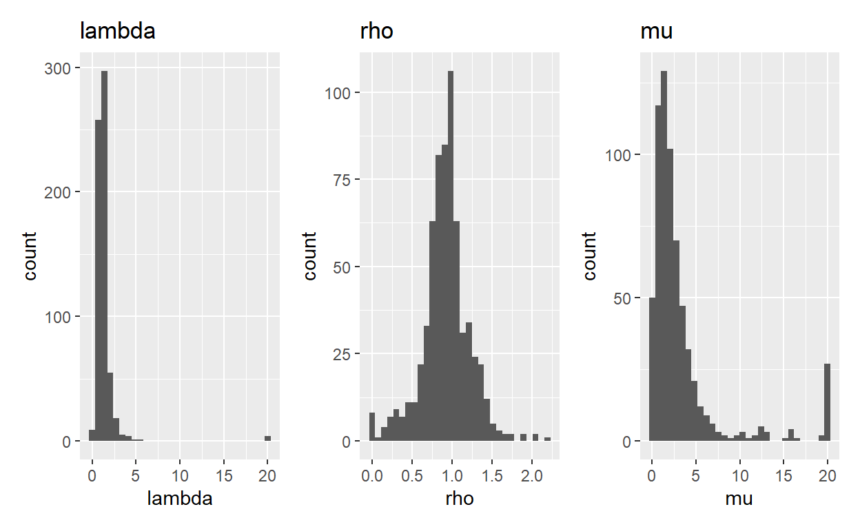
Figure 5: Histograms of lambda, rho, and mu when using multiple starting points and added constraints (lower = .01, .01, .01, upper = 20, 10, 20, respectively).
Between rerunning the models with multiple starting points and incorporating new constraints onto our parameters, our histograms look a lot more sensible.
Evaluating model predictions
Last thing we’ll do is to see how our model does at capturing our data. There are multiple ways of doing this, but one of the most straightforward is to see how often each participants’ parameters correctly predicted their choice. To do this, for each participant and each trial we plug in the parameters of the participant to get the subjective utility of gain/loss/cert (Equation (1)), and use those to calculate the probability of accepting the gamble (Equation (3)): if it’s over 50%, we say the model predicts accepting, and if it’s under 50% we say the model predicts rejecting. Then, for each participant, we compare the number of gambles that the model predicts participants will accept versus the number of gambles that they actually accept – if the model were perfect, these two numbers would be the same (but of course the model won’t be perfect). This is graphed in Figure 6, where each point is a participant, and the axes correspond to how many gambles acceptances the model predicted vs. how many gamble acceptances participants actually made.
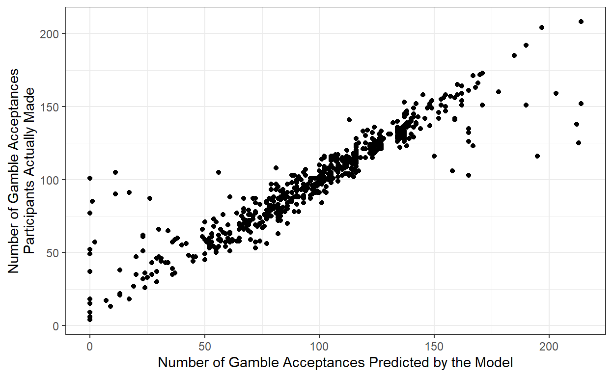
Figure 6: Number of gambles actually accepted as a function of the number of gambles the model predicts would be accepted. Each point represents a participant.
So from that, it seems like there’s a pretty tight correspondence between model predictions and actual data. Another way to look at model fit is to simply look at the percentage of trials where the model made a correct prediction – when looking at this metric, we see that the model made a correct prediction 88% of the time, which is pretty good.
And that’s it! We’ll talk next time about model comparison in the context of delay discounting, and then down the line we’ll talk about doing this in a hierarchical bayesian way, which is definitely cooler. Below I’ve reproduced all the code you need to run everything:
Full Code
Setup for the analysis:
library(tidyverse)

# calculate subjective utility given lambda/rho
# takes a vector of values and returns subjective utility
calc_subjective_utility <- function(vals, lambda, rho) {
  ifelse(vals >= 0, vals^rho, -lambda * ((-vals)^rho))
}

# calculate utility difference from vectors of gains,
# losses, and certainty
calc_utility_diff <- function(su_gain, su_loss, su_cert) {
  (.5*su_gain + .5*su_loss) - su_cert
}

# calculate the probability of accepting a gamble,
# given a difference in subjective utility and mu
calc_prob_accept <- function(gamble_cert_diff, mu) {
  (1 + exp(-mu * (gamble_cert_diff)))^-1
}


# Function to minimize with optim:
minimize_LL_prospect <- function(df, par) {
  # takes as input par, which is expected to be of the form c(lambda, rho, mu)
  # takes also a dataframe of gambles and choices (in this example, our single subject)
  lambda_par <- par[1]
  rho_par <- par[2]
  mu_par <- par[3]
  df_updated <- df %>%
    # (mutate = add variables)
    mutate(
      # Step 2: calculate subjective utility:
      cert_su = calc_subjective_utility(cert, lambda_par, rho_par),
      loss_su = calc_subjective_utility(loss, lambda_par, rho_par),
      gain_su = calc_subjective_utility(gain, lambda_par, rho_par),
      # Step 3: calculate the difference in
      # subjective utility between choices
      gamble_cert_diff = calc_utility_diff(gain_su, loss_su, cert_su),
      # Step 4: calculate the probability of accepting
      prob_accept = calc_prob_accept(gamble_cert_diff, mu = mu_par),
      # Recode the probability of acceptance, such that if it's 1, subtract
      # a very small amount, and if it's 0 add a very small amount"
      prob_accept_rc = case_when(prob_accept == 1 ~ 1-.Machine$double.eps,
                                 prob_accept == 0 ~ 0+.Machine$double.eps,
                                 TRUE ~ prob_accept),
      # Step 5: calculate log likelihood
      log_likelihood_trial = took_gamble*log(prob_accept_rc) +
        (1-took_gamble)*log(1-prob_accept_rc))

  -sum(df_updated$log_likelihood_trial)
}
Running for each participant using `nest’ and ‘map’:
data_nested <- data_clean %>%
  nest(data = -c(study, subject))

library(furrr)
future::plan(multisession, workers = 4) # set workers to the number of cores in your processor
# if you don't want to run 4 different starting points, you can delete optim_out_2 through _4.
data_optim_quad <- data_nested %>%
  mutate(optim_out_1 = future_map(data, ~ optim(par = c(1.24, .83, 2.57),
                                               fn = minimize_LL_prospect,
                                               df = .,
                                               method = 'L-BFGS-B',
                                               lower = c(.01,.01,.01),
                                               upper = c(20, 10, 20))),
         optim_out_2 = future_map(data, ~ optim(par = c(1, 1, 1),
                                               fn = minimize_LL_prospect,
                                               df = .,
                                               method = 'L-BFGS-B',
                                               lower = c(.01,.01,.01),
                                               upper = c(20, 10, 20))),
         optim_out_3 = future_map(data, ~ optim(par = c(2, 1, .9),
                                               fn = minimize_LL_prospect,
                                               df = .,
                                               method = 'L-BFGS-B',
                                               lower = c(.01,.01,.01),
                                               upper = c(20, 10, 20))),
         optim_out_4 = future_map(data, ~ optim(par = c(1.5, .83, 4.22),
                                               fn = minimize_LL_prospect,
                                               df = .,
                                               method = 'L-BFGS-B',
                                               lower = c(.01,.01,.01),
                                               upper = c(20, 10, 20))))
# function that takes a list of models and returns the one with lowest LL of the set that converged
evaluate_model <- function(model_list) {
  names(model_list) <- str_c('m', 1:length(model_list))
  models_tibble <- as_tibble(model_list)

  convergence_mat <- models_tibble %>%
    summarise(across(everything(), ~ map_dbl(., 'convergence')))
  ll_mat <- models_tibble %>%
    summarise(across(everything(), ~ map_dbl(., 'value')))

  ll_mat[convergence_mat != 0] <- NA
  lowest_likelihood <- apply(ll_mat, 1, which.min)

  index_mat <- matrix(c(1:nrow(models_tibble), lowest_likelihood), ncol = 2, byrow=FALSE)
  as.matrix(models_tibble)[index_mat]
}

# extract the parameters from the best fitting model
data_optim_quad_pars <- data_optim_quad %>%
  mutate(best_model = evaluate_model(list(optim_out_1, optim_out_2, optim_out_3, optim_out_4)),
         convergence = map_dbl(best_model, 'convergence'),
         pars = map(best_model, 'par'),
         lambda = map_dbl(pars, ~ .[1]),
         rho = map_dbl(pars, ~ .[2]),
         mu = map_dbl(pars, ~ .[3]))
Running the above code using a for loop instead of map
data_for_loop <- data_clean %>% mutate(study_subject = str_c(study, subject, sep = '_'))

unique_subjects <- unique(data_for_loop$study_subject)

optim_output_1 <- vector(mode = "list", length = length(unique_subjects))
optim_output_2 <- vector(mode = "list", length = length(unique_subjects))
optim_output_3 <- vector(mode = "list", length = length(unique_subjects))
optim_output_4 <- vector(mode = "list", length = length(unique_subjects))

for (i in 1:length(unique_subjects)) {
  data_subject <- data_for_loop %>% filter(study_subject == unique_subjects[i])

  optim_output_1[i] = list(optim(par = c(1.24, .83, 2.57),
                            fn = minimize_LL_prospect,
                            df = data_subject,
                            method = 'L-BFGS-B',
                            lower = c(.01,.01,.01),
                            upper = c(20, 10, 20)))
  optim_output_2[i] = list(optim(par = c(1, 1, 1),
                            fn = minimize_LL_prospect,
                            df = data_subject,
                            method = 'L-BFGS-B',
                            lower = c(.01,.01,.01),
                            upper = c(20, 10, 20)))
  optim_output_3[i] = list(optim(par = c(2, 1, .9),
                            fn = minimize_LL_prospect,
                            df = data_subject,
                            method = 'L-BFGS-B',
                            lower = c(.01,.01,.01),
                            upper = c(20, 10, 20)))
  optim_output_4[i] = list(optim(par = c(1.5, .83, 4.22),
                            fn = minimize_LL_prospect,
                            df = data_subject,
                            method = 'L-BFGS-B',
                            lower = c(.01,.01,.01),
                            upper = c(20, 10, 20)))
}

output_tibble <- tibble(study_subject = unique_subjects,
                        optim_out_1 = optim_output_1,
                        optim_out_2 = optim_output_2,
                        optim_out_3 = optim_output_3,
                        optim_out_4 = optim_output_4)


# function that takes a list of models and returns the one with lowest LL of the set that converged
evaluate_model <- function(model_list) {
  names(model_list) <- str_c('m', 1:length(model_list))
  models_tibble <- as_tibble(model_list)

  convergence_mat <- models_tibble %>%
    summarise(across(everything(), ~ map_dbl(., 'convergence')))
  ll_mat <- models_tibble %>%
    summarise(across(everything(), ~ map_dbl(., 'value')))

  ll_mat[convergence_mat != 0] <- NA
  lowest_likelihood <- apply(ll_mat, 1, which.min)

  index_mat <- matrix(c(1:nrow(models_tibble), lowest_likelihood), ncol = 2, byrow=FALSE)
  as.matrix(models_tibble)[index_mat]
}

# extract the parameters from the best fitting model
data_optim_quad_pars <- output_tibble %>%
  mutate(best_model = evaluate_model(list(optim_out_1, optim_out_2, optim_out_3, optim_out_4)),
         convergence = map_dbl(best_model, 'convergence'),
         pars = map(best_model, 'par'),
         lambda = map_dbl(pars, ~ .[1]),
         rho = map_dbl(pars, ~ .[2]),
         mu = map_dbl(pars, ~ .[3]))
Acknowledgments
This post was greatly improved thanks to helpful comments from Andrew Alexander, Ryan Carlson, Nathaniel Haines, David Melnikoff, and Guy Voichek.
Technically they were concerned with violations of Expected Utility Theory – an economic model of rational decision-making – which is a more nuanced version of expected value. If you’re interested in the details, I highly recommend both of the Kahneman and Tversky articles cited in this paragraph.↩︎
Technically, gains and losses are relative to some reference point – in these examples that will always be $0, but there are many cases where the reference point is not $0. K&T also discuss how probability weights vary, but we’re not going to get into that.↩︎
Like everything in R, there are a bunch of fancy packages that include different types of maximum-likelihood estimators. We will be using the one available in base R. If you want to get fancy, I recommend using hierarchical Bayesian modeling via the hBayesDM package↩︎
very likely this parameter is on its way to negative infinity↩︎
The elegant way to do this is with the debugger, the inelegant way is to just add the line
print(par)at the beginning of the minimize_LL_prospect_v1 function. I’ll leave it to the reader to guess which one I used here.↩︎These come from my data: I clustered the data and took the centers of the most populous clusters↩︎